How to Work with Large Geospatial Datasets: 10 Best Practices That Scale

Governance, a shared data catalogue, and early stakeholder alignment decide whether a sound platform actually gets used.Most teams don’t set out to build a geospatial data platform. They start with a shapefile, then a folder of shapefiles, then a database that used to be fast, and at some point the tools that worked at 2GB simply stop working at 200GB. This article lays out tips for managing large geospatial datasets at every stage of that growth curve: what actually breaks first, which storage formats and compute engines to reach for at each size threshold, how to control cloud costs as volume grows, and how to keep technical and non-technical teams aligned along the way.

The goal isn’t to hand you a list of tools. It’s a decision framework, architecture, indexing strategy, and cost model in one place, so you can match your stack to your data instead of guessing.

What Counts as “Large” Geospatial Data (and Where Traditional Tools Break)

“Large” isn’t one number. It’s a series of thresholds where a familiar tool quietly stops working. A shapefile caps out at 2GB per .shp or .dbf file (4GB combined), so exports beyond that fail or silently truncate. Desktop GIS tools like QGIS start lagging on rendering and attribute joins once a single machine’s RAM is doing double duty as your database. And PostGIS, while capable well into the billions of rows with the right indexing, starts showing query times measured in minutes instead of seconds once tables aren’t partitioned and spatial indexes aren’t tuned.

The practical rule: if you’re asking “why is this suddenly slow,” you’ve already crossed a threshold. The fix is rarely a faster machine, it’s usually a format, index, or architecture change.

The 10 Best Practices That Scale

These ten practices aren’t a flat checklist, they’re grouped into five categories that map to how a geospatial stack actually gets built: the storage layer, spatial indexing and partitioning, processing and compute, cost optimization, and governance and stakeholder alignment. Work through them roughly in that order, since each category sets up the one after it.

A. Get the Storage Layer Right

Three of the ten practices below live at the storage layer, since getting this right removes most downstream performance problems before they start.

1. Move to cloud object storage.
   S3, Google Cloud Storage, or Azure Blob give you durability, HTTP range request support (so tools can read only the bytes they need), and pricing that scales down as data ages. As of 2026, standard hot storage runs roughly $0.018 to $0.023 per GB per month depending on provider, with archive tiers as low as $0.001 per GB per month for data you rarely touch.
   
   
2. Choose a cloud-native format instead of shapefile or raw GeoJSON.
   This is the single highest-leverage decision in your stack, and it’s the one most teams get wrong by default.
   
   

GeoParquet applies columnar compression by default, which typically shrinks datasets several times over versus uncompressed GeoJSON, with no separate zip step needed. For read-heavy analytics, that’s compute savings on every query, not just storage savings.

3. Add a table format for versioning.
   Apache Iceberg or Delta Lake sit on top of your object storage and give you snapshotting, schema evolution, and safe concurrent writes, so a bad ingestion job doesn’t corrupt months of history. This is the same principle SafeGraph’s engineering team has recommended since the format’s early days: cloud storage plus a table format lays the foundation for everything that runs on top of it.

B. Spatial Indexing and Partitioning

This is where most large-dataset projects either become fast or stay slow, and it’s the part most competing guides skip entirely.

4. Use spatial indexes: H3, S2, and R-tree/quadtree.
   Uber’s H3 divides the globe into hexagonal cells across 16 resolution levels, and its uniform neighbor distances make it well suited to mobility, demand heatmaps, and proximity analysis. Google’s S2 uses a quadtree decomposition into quadrilateral cells across 31 levels, optimized for 64-bit integer operations, and is the backbone of large-scale systems like Google Maps.
   
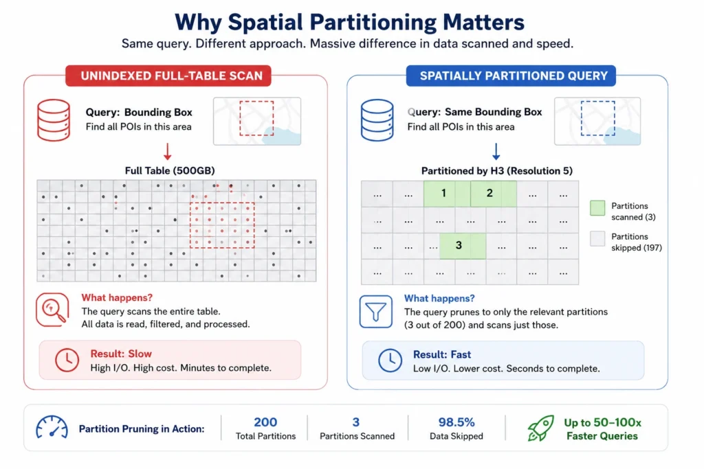
   Neither is strictly better: H3 tends to win when you need uniform neighborhoods (drive-time bands, catchment areas), while S2 tends to win when you need fine-grained precision at web scale. For transactional spatial databases, PostGIS’s default GiST index (a variant of an R-tree) remains the right choice, and quadtrees are common in file-level formats like FlatGeobuf, where a packed index travels with the data itself.
   
   
5. Partition your data spatially in Parquet.
   Partitioning GeoParquet files by a coarse spatial key (an H3 cell at a low resolution, or a geohash prefix) means a query with a bounding box only reads the partitions that could possibly match, instead of scanning the entire dataset. On a 500GB POI table, this is routinely the difference between a query that finishes in seconds and one that finishes in minutes.
   
   

C. Choosing Tools by Dataset Size

Rather than listing every tool, match your stack to where your data actually sits today, not where you think it might be in three years.

D. Processing and Compute

Pick compute based on where your data sits in the table above, then scale up only when you hit the ceiling of your current tier.

• Match your compute engine to your data’s scale.
  Single-machine tools like DuckDB Spatial or GeoPandas handle up to roughly medium-sized datasets comfortably. Dask extends that same GeoPandas-style workflow across multiple cores or a small cluster without the operational overhead of a full distributed system, a good middle step before committing to Spark.
  
  For genuinely massive datasets, Apache Sedona extends Spark (and now Flink and Snowflake) with 300+ spatial functions and native support for GeoParquet, Shapefile, GeoJSON, and PostGIS; SedonaDB, released in 2025 as a single-node companion engine, now also supports GPU-accelerated spatial joins for teams that need distributed-grade performance without a full cluster.
  
  If your team already lives in a cloud warehouse, BigQuery and Snowflake both support native geography types, often the fastest path to production without managing a separate compute layer.
  
  
• Query data in place instead of importing it first.
  DuckDB Spatial can query GeoParquet files sitting on S3 without an import step, reading only the columns and row groups a given query needs through HTTP range requests. Querying cloud storage directly, rather than pulling everything into a database first, holds up even on datasets far larger than your local machine’s memory, and it removes an entire ETL step most teams don’t realize they can skip.
  
  

E. Cost Optimization

8. Balance preprocessing with on-demand compute.
   The biggest cost lever isn’t storage tier, it’s how much you preprocess versus compute on demand. Rayne Gaisford, Head of Data Strategy and Equity Research at Jefferies, and Felix Cheung, SafeGraph’s VP of Engineering, have both pointed to the same tradeoff in practice: teams that pre-canned every possible output ended up paying for compute nobody used, while teams that computed everything on demand paid a latency tax on every question.
   
   

Hear Gaisford and Cheung walk through this tradeoff in detail: watch the full webinar on best practices for working with large quantities of geospatial data.

A worked example: running a nightly batch job on a 10-node cluster of r5.4xlarge instances (roughly $1.008 per hour per node as of mid-2026) for 12 hours costs about $121 per day, or roughly $3,630 a month, regardless of whether every output gets used. Shifting to an incremental model, where only changed partitions are reprocessed in a targeted 3-hour window, cuts that to around $907 a month on the same cluster, a rough 75% reduction, with the tradeoff that a handful of ad hoc queries run a little slower. For most teams, that trade is worth it: the marginal queries are rare, and the savings compound every month.

Storage costs follow the same logic. Cloud-native formats like GeoParquet often cut raw storage several times over compared to uncompressed shapefile or GeoJSON, and tiering older, rarely-queried data into cold or archive storage classes (as low as $0.001 per GB per month) adds further savings with no query-time cost for data you’re not actively using.

F. Governance and Stakeholder Alignment

A technically sound stack still fails if nobody can find the data or agree on who owns it. Two practices matter most here.

9. Maintain a central data catalogue.
   As organizations grow past a handful of teams, an active data catalogue committee (not just a wiki page) keeps different groups from duplicating datasets or working from stale versions. This is less about tooling and more about assigning clear ownership: someone needs to be accountable for each dataset’s freshness and accuracy, not just its existence.
   
   
10. Align with non-technical stakeholders before you build.
    The first job of any team building on geospatial data is translating a business question into a data question, and that conversation needs to happen before pipelines get built, not after. Establishing a shared vocabulary early means you can reuse it on the next request instead of starting from zero each time, and it means one team’s data catalogue can often answer another team’s question without a new pipeline at all.
    
    

These two practices, cataloguing and stakeholder alignment, are the foundation of a broader five-phase framework. For the full 5-phase strategy framework, including metadata standards and performance metrics for tracking data health over time, see our geospatial data management guide.

Worked Example: Loading and Querying a Large POI Dataset

Say you’re working with a national points-of-interest dataset, several million records with brand, category, and location attributes, stored as partitioned GeoParquet on S3. The workflow looks like this:

1. Land the raw data in an S3 bucket, partitioned by a coarse H3 cell or state/region code.
   
   
2. Register a table format (Iceberg or Delta) on top so you can snapshot before and after each ingestion run.
   
   
3. Query directly with DuckDB Spatial for exploratory work, or point Apache Sedona at the same partitions for a distributed join against a larger dataset, like matching each POI to a building footprint.
   
   
4. Serve the result as PMTiles if the output is a map, or write it back to GeoParquet if the output feeds another pipeline.
   
   

This pattern holds regardless of the specific POI source. Datasets like SafeGraph’s Places data (point-level business attributes) and Geometry data (building footprints) are commonly used for exactly this kind of input, joined against internal datasets rather than analyzed in isolation.

Reference Architecture

Putting it all together, a reference architecture for large geospatial data looks like this:

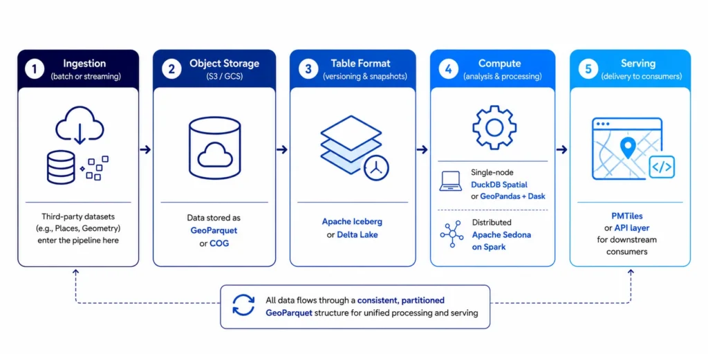
Ingestion (batch or streaming) → Object storage (S3/GCS, data written as GeoParquet or COG) → Table format (Iceberg or Delta Lake for versioning and snapshots) → Compute (DuckDB Spatial or GeoPandas+Dask for single-node work, Apache Sedona on Spark for distributed work) → Serving (PMTiles or an API layer for downstream consumers).

Third-party datasets, like Places or Geometry data, typically enter this pipeline at the ingestion stage, get normalized into the same partitioned GeoParquet structure as internal data, and flow through the same compute and serving layers from there. That consistency is what makes a stack maintainable as more data sources get added over time.

Closing Thoughts

None of this requires adopting every tool at once. The teams that manage large geospatial datasets well are the ones that match their stack to their current data size, revisit that match as volume grows, and treat indexing and governance as part of the architecture rather than an afterthought. Start with the threshold table at the top of this article, find where your data sits today, and build from there.